What makes data difficult for a language model?

I recently pre-trained a small language model from scratch for the first time.

The model was trained on a mixture of data sources. Besides the overall loss, I tracked the loss of each source separately, and one pattern was hard to miss: structured, repetitive domains such as code and algebra converged quickly to low loss, while heterogeneous web text stayed noticeably higher.

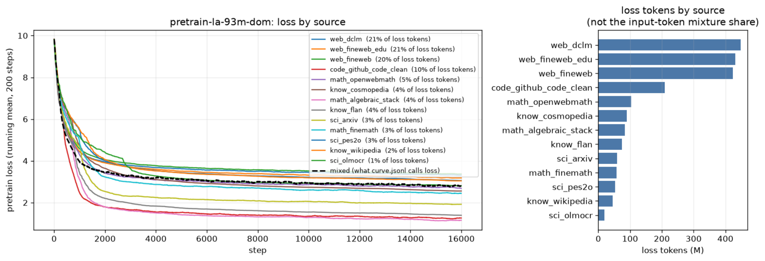Left: training loss per source (200-step running mean) over 16k steps of my small pre-training run; the dashed line is the mixed loss a single training curve would report. Right: how many loss tokens each source contributed, which is not the same as its input mixture share.

A few things stand out in this first run:

• Code and algebra go lowest. math_algebraic_stack ends near 1.2 and code_github_code_clean near 1.3, and both drop below 2 within roughly the first 1,500 steps.
• Web text stays highest. The three web sources, which together make up about 62% of loss tokens, plateau somewhere around 3.1-3.4.
• “Math” is not one difficulty. math_openwebmath, which is math written as web prose, stays near 2.7, far above math_algebraic_stack. Same topic, very different loss, which already hints that format matters more than subject.
• Templated data is easy too. know_flan, built from instruction templates, sits near 1.4, close to code.
• The mixed loss hides all of this. The single dashed curve (about 2.8) is dominated by web text simply because web contributes most of the tokens.

These are training-loss curves from one run, not held-out evaluations, so I treat them as a hint rather than a measurement.

It is tempting to read this as “the model is good at code and bad at web text.” I do not think that reading is justified yet. This post is a note on why, and on the experiment I want to run next.

Human difficulty is not predictive difficulty

What is difficult for a person and what is difficult for next-token prediction can be very different things.

Math and code are often conceptually hard for us. But their syntax and regular structure constrain what can come next. After for i in range(, the plausible continuations are few. A closing bracket, an indentation level, or the next step of a routine derivation is often nearly determined by the context.

Ordinary web text looks easy to read, yet it leaves many more doors open. After “I went to the store and”, a large number of continuations are reasonable, and no amount of modeling skill can make that choice certain.

So a low loss on code may say less about how well the model understands code and more about how narrow the next-token distribution of code is.

Loss mixes two different things

A small identity makes this concrete. For a context \(x\), let \(p(\cdot \mid x)\) be the true next-token distribution and \(q(\cdot \mid x)\) the model’s prediction. The expected cross-entropy loss splits into two parts:

The first term is a property of the data. The second term is the gap that training can close. A per-domain loss curve reports only their sum.

In simple words - Entropy vs. loss: Entropy is how uncertain the next token really is. Loss is how surprised the model was. A domain can have high loss simply because its next tokens are genuinely unpredictable, even when the model has learned almost everything that can be learned from it.

Under that view, “code converged lower than web text” has at least two explanations that a raw loss curve cannot separate:

1. code has lower intrinsic entropy, so its floor is lower; or
2. the model genuinely closed more of the learnable gap on code.

Both may be true at once. The interesting quantity is the second one, and it is the one I have not measured.

Existing work points in the same direction

This is not a new concern, and several lines of work already treat it seriously.

• DoReMi (Xie et al., 2023) optimizes domain weights with excess loss: the loss of a proxy model minus the loss of a reference model on the same domain. Subtracting the reference roughly removes each domain’s intrinsic difficulty, so the optimizer attends to domains where there is still something to learn instead of domains that are simply noisy.
• Rho-1 (Lin et al., 2024) looks at loss at the token level and finds that tokens follow very different trajectories during training: some are learned early, some stay hard, and some fluctuate. Averaging them into one number hides most of that structure.
• Entropy-Guided Token Dropout (arXiv:2512.23422) reports that, in multi-epoch training on limited domain data, low-entropy tokens are learned quickly and come to dominate optimization, while generalization on high-entropy tokens degrades with continued training.
• Data Mixing Laws (Ye et al., 2024) show that domain-level loss can be predicted as a function of the mixture proportions, which suggests these differences are systematic enough to model rather than noise.

Together they suggest that “difficulty” is better defined relative to what is learnable, and better measured at the token level than at the domain level.

The next experiment

Instead of comparing raw loss across domains, I want to measure the relationship between token-level predictability and how fast each token is learned.

1. Estimate predictability with a reference model

The true entropy \(H(p)\) is not observable. As a proxy, I will score a held-out set with a larger, well-trained reference model and record, for every token:

• predictive entropy: the entropy of the reference model’s full next-token distribution, \(H(q_{\text{ref}}(\cdot \mid x))\), which says how open the context is;
• reference surprisal: \(-\log q_{\text{ref}}(y \mid x)\) for the actual token, which says how surprising that particular token was.

These answer different questions. A context can be open (high entropy) while the observed token happens to be the most likely one, and vice versa.

2. Bucket tokens within each domain

Comparing domains mixes entropy with everything else that differs between them. So I will split tokens into entropy quantiles within each domain: the lowest-entropy tokens of web text are compared with the highest-entropy tokens of web text, and the same for code and algebra.

3. Track learning speed per bucket

For every saved checkpoint of my own small model, I will compute the mean loss in each bucket and summarize each curve with:

• time to converge: the number of training tokens needed to close, say, 90% of the gap between the initial and final bucket loss;
• excess loss: the small model’s loss minus the reference model’s loss, following the DoReMi idea, at every checkpoint.

If difficulty is mostly entropy, the curves should line up by entropy bucket regardless of domain. If they do not, something about the domain itself is doing work that entropy does not explain.

4. Controls I need to watch

• Tokenization: code and math are tokenized very differently from prose, and a “token” may carry different amounts of information in each domain.
• Duplication and boilerplate: licenses, imports, and templated pages can produce near-zero loss by memorization rather than learning.
• Position in the sequence: tokens late in a long context are usually easier, and domains differ in document length.
• Reference-model bias: the reference model has its own training mixture, so its entropy estimates are not a neutral ground truth.

Questions I want the data to answer

• Within a single domain, are low-entropy tokens learned faster, and by how much?
• Does the gap in learning speed between domains shrink once entropy is held fixed?
• Is there a group of high-entropy tokens whose excess loss keeps falling late in training? Those may be where the “hard” learning actually happens.
• Would a mixture chosen by excess loss rather than raw loss change what my small model ends up being good at?

I do not have answers yet. The per-domain curve was only the first hint that “difficulty” needs a sharper definition.

It is striking that pre-training has become accessible enough for an individual to run a model from scratch and then ask questions like these with a relatively small experiment. I will follow up with the results.

Key terms

• Per-domain loss: the average next-token loss measured on data from a single source.
• Entropy: how spread out the next-token distribution is; the part of the loss no model can remove.
• Surprisal: \(-\log q(y \mid x)\) for the token that actually appeared.
• Excess loss: a model’s loss minus a reference model’s loss on the same data, used as a proxy for what is still learnable.
• Data mixture: the proportion of each source in the pre-training corpus.

한국어

처음으로 작은 언어 모델을 처음부터 pre-training 해봤습니다.

여러 데이터 소스를 섞어 학습하면서 전체 loss뿐 아니라 source별 loss를 따로 추적해봤는데, 꽤 뚜렷한 차이가 보였습니다. Code나 algebra처럼 구조적이고 반복적인 패턴이 있는 데이터는 빠르게 낮은 loss로 수렴한 반면, 일반적인 web corpus는 상대적으로 높은 loss를 유지했습니다.

위 그래프에서 math_algebraic_stack과 code_github_code_clean은 약 1.2-1.3까지 내려가지만, loss token의 약 62%를 차지하는 세 개의 web source는 3.1-3.4 근처에서 멈춥니다. 특히 같은 “수학”이라도 web 문서 형태인 math_openwebmath는 약 2.7에 머물러, 주제보다 형식이 loss를 더 크게 좌우한다는 힌트를 줍니다. 템플릿 기반인 know_flan도 1.4 근처로 code와 비슷하게 낮습니다. 그리고 하나의 mixed loss(약 2.8)만 보면 이런 차이가 대부분 web text에 가려집니다. 다만 이는 한 번의 run에서 나온 training loss이므로 결론이 아니라 힌트로 보고 있습니다.

여기서 흥미로운 질문이 하나 생겼습니다.

언어 모델에게 데이터가 “어렵다”는 것은 정확히 무엇일까?

사람에게 어려운 내용과 next-token prediction 관점에서 어려운 데이터는 전혀 다를 수 있습니다. 수학이나 코드는 사람에게 어려울 수 있지만, syntax와 반복적인 structure 때문에 다음 token의 conditional distribution은 오히려 좁을 수 있습니다. 반대로 평범한 web text는 내용 자체는 쉬워 보여도 가능한 다음 token의 분포가 훨씬 넓을 수 있습니다.

실제로 우리가 측정하는 cross-entropy loss는 데이터 자체의 irreducible entropy와 모델이 아직 배우지 못한 부분(KL divergence)의 합입니다. 그래서 code의 loss가 낮다는 사실만으로는 “모델이 code를 더 잘 배웠다”와 “code의 다음 token이 원래 더 예측 가능하다”를 구분할 수 없습니다. 지금의 관찰은 결론이 아니라, difficulty를 더 정확하게 정의해야 한다는 첫 번째 힌트에 가깝습니다.

관련 연구도 같은 방향을 가리킵니다. DoReMi는 domain마다 intrinsic difficulty가 다르기 때문에 raw loss 대신 reference model 대비 excess loss를 사용합니다. Rho-1은 token마다 학습 궤적이 크게 다르다는 점을 보여주고, 최근 연구에서는 제한된 domain 데이터로 여러 epoch 학습할 때 low-entropy token이 빠르게 학습되어 optimization을 지배한다는 현상이 보고되었습니다. Data Mixing Laws는 데이터 mixture와 domain별 loss 사이에 예측 가능한 관계가 있음을 보여줍니다.

그래서 다음 실험에서는 단순히 domain별 loss를 비교하는 대신 token-level entropy / predictability ↔ training loss의 관계를 직접 측정해보려고 합니다.

1. 더 큰 reference model로 각 token의 predictive entropy와 surprisal을 계산합니다.
2. 같은 domain 안에서 token을 entropy 구간별로 나눕니다.
3. 제 작은 모델의 checkpoint마다 구간별 loss를 계산해, 각 구간이 얼마나 빨리 수렴하는지와 reference 대비 excess loss가 어떻게 변하는지 봅니다.
4. tokenizer 차이, 중복·boilerplate, sequence 내 위치, reference model 자체의 bias는 따로 통제해야 할 변수로 둡니다.

알고 싶은 질문은 이렇습니다. 같은 domain 안에서 low-entropy token은 얼마나 더 빨리 학습될까? entropy를 고정하면 domain 간 차이는 줄어들까? 학습 후반까지 excess loss가 계속 줄어드는 high-entropy token 그룹이 있다면, 그곳이 진짜 “어려운” 학습이 일어나는 곳일까?

아직 답은 없습니다. 다만 개인이 직접 pre-training을 돌려보고 이런 질문까지 실험해볼 수 있다는 것 자체가 꽤 재미있는 시대라는 생각이 듭니다. 결과가 나오면 이어서 정리해보겠습니다.