Study of MobileNet and basic information and coding of Cov2d, Forward propagation, BN, Quantized, etc…
MobileNet

MobileNet if from Google, which was aimed for using mobile or cpu based computer machine learning in realtime. Key idea of this paper is reducing convolution layer by detphwise seperable convolution. This is not first offered in this paper. Originally it was from Google’s Xception

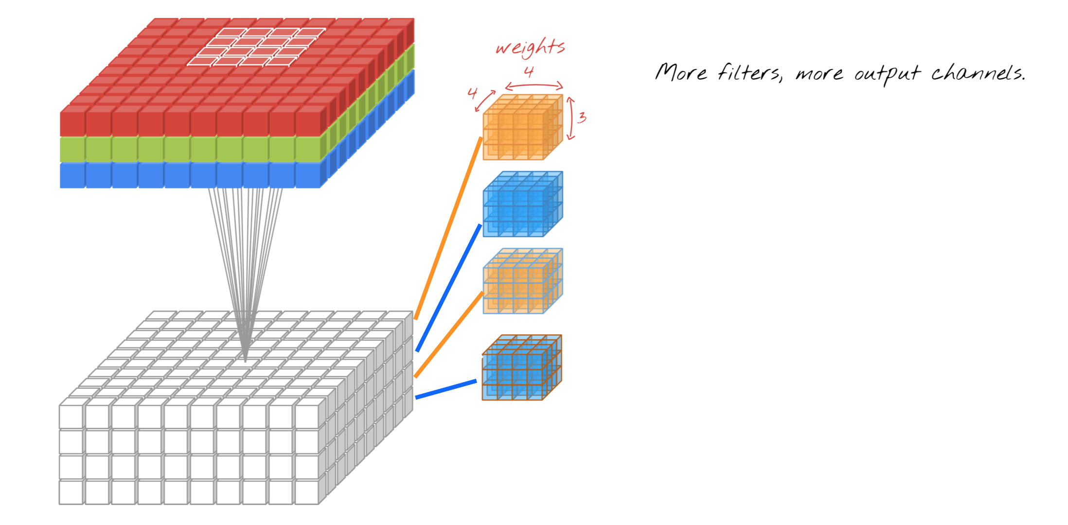
MobileNet used only one pooling and one stride for convolutional neural network. Now we can evaluate the process cost by counting how many calculation need per one convolution repective to standard convolution and depthwise convolution.
Basic iteration formula will be \(G_{k,l,n} = \sum_{i,j,m} K_{i,j,m,n} \cdot F_{k+i-1,l+j-1,m}\)

For the standard cost of convolutions will be \(D_{K} \cdot D_{K} \cdot M \cdot N \cdot D_{F} \cdot D_{F}\)
Which \(D_{K}\), \(D_{F}\), \(M\), \(N\) represent kernel, feature map size, input channel depth and kernel channel depth, and kernel outputnumber which is feature output number
However depthwise convolution cost will be
\[(D_{K} \cdot D_{K} \cdot M + M \cdot N) \cdot D_{F} \cdot D_{F}\] \[\frac{New Cost}{Original Cost} = \frac{(D_{K} \cdot D_{K} \cdot M + M \cdot N) \cdot D_{F} \cdot D_{F}}{D_{K} \cdot D_{K} \cdot M \cdot N \cdot D_{F} \cdot D_{F}} = \frac{1}{D^2_{k}} + \frac{1}{N}\]Most of the kernel size is 3 by 3 therefore it lessen 1/9 times of parameters
For each process of convoultion + ReLu and Max pooling of original image. The result of data gets more sharper than original data.

Question: does MobileNet also applies for both training and testing process?
Basic Code of Back Propogation Including Concepts of Pooling
import numpy as np, sys

from scipy.ndimage.filters import maximum_filter
import skimage.measure
from scipy.signal import convolve2d

np.random.seed(7839)

x1 = np.array([
    [1, 1, 0, 1, 0, 1],
    [1, 1, 0, 1, 0, 1],
    [1, 1, 0, 1, 0, 1],
    [1, 1, 1, 1, 0, 1],
    [1, 1, 1, 1, 0, 1],
    [1, 1, 1, 1, 0, 1]
])

x2 = np.array([
    [-1, 0, -1, 0, 0, 1],
    [-1, 0, -1, 0, 0, 1],
    [-1, 0, -1, 1, 0, 1],
    [-1, -1, -1, 0, 0, -1],
    [-1, 0, -1, 0, 0, -1],
    [-1, 0, -1, 0, 0, -1]
])
X = np.array([x1, x2])
y = np.array([
    [x1.sum()],
    [x2.sum()]
])

"""
Making channel (w1 and w2) between x and y relationship backpropagation of including Max Pool without Activation Layer
Using gradient descent algorithm
"""

num_epoch = 100
learing_rate = 0.001

w1 = np.random.randn(3, 3) * 0.66
w2 = np.random.randn(4, 1) * 5.7

prediction = np.array([])
for image_index in range(len(X)):
    current_image = X[image_index]
    current_label = y[image_index]

    print("Original Image Shape: ",current_image.shape)
    l1 = convolve2d(current_image, w1, mode='valid')
    print("L1 Image Shape: ",l1.shape)
    l1M = skimage.measure.block_reduce(l1, (2, 2), np.max)
    print("L1M Image Shape: ",l1M.shape)

    l2IN = np.reshape(l1M, (1, 4))
    l2 = l2IN.dot(w2)
    prediction = np.append(prediction, l2)

print("--- Ground Truth -----")
print(y.T)
print("--- Before Training -----")
print(prediction.T)

for iter in range(num_epoch):

    for image_index in range(len(X)):
        current_image = X[image_index]
        current_label = y[image_index]

        # print("Original Image Shape: ",current_image.shape)
        l1 = convolve2d(current_image, w1, mode='valid')
        # print("L1 Image Shape: ",l1.shape)
        l1M = skimage.measure.block_reduce(l1, (2, 2), np.max)
        # print("L1M Image Shape: ",l1M.shape)

        l2IN = np.reshape(l1M, (1, 4))
        l2 = l2IN.dot(w2)

        cost = np.square(l2 - current_label).sum() * 0.5
        # print("Current Iter: ", iter, " current cost :", cost ,end='\r')

        grad_2_part_1 = l2 - current_label
        grad_2_part_3 = l2IN
        grad_2 = grad_2_part_3.T.dot(grad_2_part_1)

        grad_1_part_1 = np.reshape((grad_2_part_1).dot(w2.T), (2, 2))
        grad_1_mask = np.equal(l1, l1M.repeat(2, axis=0).repeat(2, axis=1)).astype(int)
        # print("\nCoordinate of Max Pooling - Blue Numbers : \n",grad_1_mask)

        # print("\nOriginal Gradient: \n",grad_1_part_1)
        grad_1_window = grad_1_part_1.repeat(2, axis=0).repeat(2, axis=1)
        # print("\nHere is the secret of Performing Element Wise Multiplication : \n",grad_1_window)

        grad_1_part_1 = grad_1_mask * grad_1_window
        # print("\nAfter Element Wise Multiplication : \n",grad_1_part_1)
        # sys.exit()

        grad_1_part_3 = current_image
        grad_1 = np.rot90(convolve2d(grad_1_part_3, np.rot90(grad_1_part_1, 2), mode='valid'), 2)

        w2 = w2 - learing_rate * grad_2
        w1 = w1 - learing_rate * grad_1

prediction = np.array([])
for image_index in range(len(X)):
    current_image = X[image_index]
    current_label = y[image_index]

    # print("Original Image Shape: ",current_image.shape)
    l1 = convolve2d(current_image, w1, mode='valid')
    # print("L1 Image Shape: ",l1.shape)
    l1M = skimage.measure.block_reduce(l1, (2, 2), np.max)
    # print("L1M Image Shape: ",l1M.shape)

    l2IN = np.reshape(l1M, (1, 4))
    l2 = l2IN.dot(w2)
    prediction = np.append(prediction, l2)

print("--- Ground Truth -----")
print(y.T)
print("--- After Training -----")
print(prediction.T)
Reference
Github
MobileNet에 대한 공부와 기본 정보, 그리고 Cov2d, Forward propagation, BN, Quantized 등의 코딩을 정리합니다.
MobileNet
MobileNet은 Google에서 나온 모델로, 모바일 또는 CPU 기반 컴퓨터에서 실시간으로 머신러닝을 사용하는 것을 목표로 했습니다. 이 논문의 핵심 아이디어는 depthwise separable convolution으로 convolution layer의 연산을 줄이는 것입니다. 이는 이 논문에서 처음 제안된 것은 아니며, 원래는 Google의 Xception에서 나왔습니다.
MobileNet은 convolutional neural network에서 pooling 하나와 stride 하나만 사용했습니다. 이제 standard convolution과 depthwise convolution 각각에 대해 convolution 한 번당 필요한 연산 횟수를 세어 처리 비용을 평가할 수 있습니다.
기본 반복 수식은 다음과 같습니다. \(G_{k,l,n} = \sum_{i,j,m} K_{i,j,m,n} \cdot F_{k+i-1,l+j-1,m}\)
Standard convolution의 비용은 다음과 같습니다. \(D_{K} \cdot D_{K} \cdot M \cdot N \cdot D_{F} \cdot D_{F}\)
여기서 \(D_{K}\), \(D_{F}\), \(M\), \(N\)은 각각 kernel, feature map 크기, input channel depth(kernel channel depth), 그리고 kernel 출력 개수(즉 feature 출력 개수)를 나타냅니다.
반면 depthwise convolution의 비용은 다음과 같습니다.
\[(D_{K} \cdot D_{K} \cdot M + M \cdot N) \cdot D_{F} \cdot D_{F}\] \[\frac{New Cost}{Original Cost} = \frac{(D_{K} \cdot D_{K} \cdot M + M \cdot N) \cdot D_{F} \cdot D_{F}}{D_{K} \cdot D_{K} \cdot M \cdot N \cdot D_{F} \cdot D_{F}} = \frac{1}{D^2_{k}} + \frac{1}{N}\]대부분의 kernel 크기는 3 by 3이므로 parameter가 약 1/9 수준으로 줄어듭니다.
원본 이미지에 대해 convolution + ReLu와 Max pooling을 각각 거치면, 결과 데이터는 원본 데이터보다 더 선명해집니다.
질문: MobileNet은 training과 testing 과정 모두에 적용될까요?
Pooling 개념을 포함한 Back Propogation 기본 코드
import numpy as np, sys

from scipy.ndimage.filters import maximum_filter
import skimage.measure
from scipy.signal import convolve2d

np.random.seed(7839)

x1 = np.array([
    [1, 1, 0, 1, 0, 1],
    [1, 1, 0, 1, 0, 1],
    [1, 1, 0, 1, 0, 1],
    [1, 1, 1, 1, 0, 1],
    [1, 1, 1, 1, 0, 1],
    [1, 1, 1, 1, 0, 1]
])

x2 = np.array([
    [-1, 0, -1, 0, 0, 1],
    [-1, 0, -1, 0, 0, 1],
    [-1, 0, -1, 1, 0, 1],
    [-1, -1, -1, 0, 0, -1],
    [-1, 0, -1, 0, 0, -1],
    [-1, 0, -1, 0, 0, -1]
])
X = np.array([x1, x2])
y = np.array([
    [x1.sum()],
    [x2.sum()]
])

"""
Activation Layer 없이 Max Pool을 포함한 backpropagation으로 x와 y 사이의 관계를 나타내는 channel (w1, w2)을 만듭니다.
Gradient descent 알고리즘을 사용합니다.
"""

num_epoch = 100
learing_rate = 0.001

w1 = np.random.randn(3, 3) * 0.66
w2 = np.random.randn(4, 1) * 5.7

prediction = np.array([])
for image_index in range(len(X)):
    current_image = X[image_index]
    current_label = y[image_index]

    print("Original Image Shape: ",current_image.shape)
    l1 = convolve2d(current_image, w1, mode='valid')
    print("L1 Image Shape: ",l1.shape)
    l1M = skimage.measure.block_reduce(l1, (2, 2), np.max)
    print("L1M Image Shape: ",l1M.shape)

    l2IN = np.reshape(l1M, (1, 4))
    l2 = l2IN.dot(w2)
    prediction = np.append(prediction, l2)

print("--- Ground Truth -----")
print(y.T)
print("--- Before Training -----")
print(prediction.T)

for iter in range(num_epoch):

    for image_index in range(len(X)):
        current_image = X[image_index]
        current_label = y[image_index]

        # print("Original Image Shape: ",current_image.shape)
        l1 = convolve2d(current_image, w1, mode='valid')
        # print("L1 Image Shape: ",l1.shape)
        l1M = skimage.measure.block_reduce(l1, (2, 2), np.max)
        # print("L1M Image Shape: ",l1M.shape)

        l2IN = np.reshape(l1M, (1, 4))
        l2 = l2IN.dot(w2)

        cost = np.square(l2 - current_label).sum() * 0.5
        # print("Current Iter: ", iter, " current cost :", cost ,end='\r')

        grad_2_part_1 = l2 - current_label
        grad_2_part_3 = l2IN
        grad_2 = grad_2_part_3.T.dot(grad_2_part_1)

        grad_1_part_1 = np.reshape((grad_2_part_1).dot(w2.T), (2, 2))
        grad_1_mask = np.equal(l1, l1M.repeat(2, axis=0).repeat(2, axis=1)).astype(int)
        # print("\nCoordinate of Max Pooling - Blue Numbers : \n",grad_1_mask)

        # print("\nOriginal Gradient: \n",grad_1_part_1)
        grad_1_window = grad_1_part_1.repeat(2, axis=0).repeat(2, axis=1)
        # print("\nHere is the secret of Performing Element Wise Multiplication : \n",grad_1_window)

        grad_1_part_1 = grad_1_mask * grad_1_window
        # print("\nAfter Element Wise Multiplication : \n",grad_1_part_1)
        # sys.exit()

        grad_1_part_3 = current_image
        grad_1 = np.rot90(convolve2d(grad_1_part_3, np.rot90(grad_1_part_1, 2), mode='valid'), 2)

        w2 = w2 - learing_rate * grad_2
        w1 = w1 - learing_rate * grad_1

prediction = np.array([])
for image_index in range(len(X)):
    current_image = X[image_index]
    current_label = y[image_index]

    # print("Original Image Shape: ",current_image.shape)
    l1 = convolve2d(current_image, w1, mode='valid')
    # print("L1 Image Shape: ",l1.shape)
    l1M = skimage.measure.block_reduce(l1, (2, 2), np.max)
    # print("L1M Image Shape: ",l1M.shape)

    l2IN = np.reshape(l1M, (1, 4))
    l2 = l2IN.dot(w2)
    prediction = np.append(prediction, l2)

print("--- Ground Truth -----")
print(y.T)
print("--- After Training -----")
print(prediction.T)
참고 문헌
Github